Jekyll2026-02-09T18:47:56+00:00https://nandantumu.com/feed.xmlblankThe personal webpage of Nandan Tumu Zero-Shot Terrain Context Identification and Friction Estimation2025-05-18T16:00:00+00:002025-05-18T16:00:00+00:00https://nandantumu.com/blog/2025/workshop-clustering-foundation-models
Vehicles with incorrect friction estimates can lose control and even flip over.
Our approach, PC-VFE, is able to adapt to new terrain.
Click to zoom in on the poster! A high-resolution PDF version is available here
Autonomous Vehicles Must Adapt On the Fly
Traversing unknown or varying terrain is a fundamental obstacle for robust autonomous vehicle operation.
Our approach eliminates the need for pre-mapped terrain information, enabling true adaptability in new environments.
Learning Terrain Types Without Supervision
Continuous Multi-Modal Sensing The vehicle records images, state, and control data at each timestep, building a rich dataset during real operation.
Extracting Meaningful Semantic Features A Vision-Language Model (e.g., CLIP) translates images into semantic latent vectors by matching them to text-based queries. These are enhanced with basic visual features (like brightness and color) for additional context.
Unsupervised Clustering for Terrain Discovery Latent features are automatically grouped into clusters—each representing a unique, discovered terrain type – without manual labeling or prior knowledge.
Physics-Informed Optimization for Actionable Parameters For each terrain cluster, a gradient-based optimizer fine-tunes friction and related parameters, using a differentiable vehicle dynamics model to backpropagate losses from observed driving behavior.
Physics-informed optimization: 0.1 Hz (1 per 10 seconds)
Effective Control Even with Imperfect Estimation
The system autonomously distinguishes between multiple terrain types (e.g., patchy grass, dry soil, concrete, brick) in a single lap, with zero prior knowledge of the environment.
Estimated friction parameters, while not always numerically identical to ground truth, enable effective and stable control, preventing failures in simulation.
The clustering-based approach allows the controller to adapt quickly to abrupt terrain changes.
Next Steps: Toward Adaptive Off-Road Autonomy
Accelerated Context Recognition: Replace clustering with a function approximation for near-instant terrain identification.
Comprehensive System Identification: Extend to estimate all model parameters, not just friction.
Generalization: Handle an unknown number of new terrain types and maintain robust control through abrupt changes.
Takeaway: Our method demonstrates that vision-language foundation models, combined with physics-informed optimization, empower autonomous vehicles to adapt to unseen terrain in real time—without human supervision or advance mapping—unlocking new possibilities for robust off-road autonomy.
]]>Renukanandan Tumu*Multi-Modal Conformal Prediction Regions with Simple Structure by Optimizing Convex Shape Templates2024-06-22T00:00:00+00:002024-06-22T00:00:00+00:00https://nandantumu.com/blog/2024/paper-param-conf-regionMotivation
Conformal Prediction is a popular method for uncertainty quantification, resulting in prediction regions around a predictor that contain the true output with high probability. The shape of these regions, determined by a non-conformity function, can significantly impact the performance of downstream tasks in robotics.
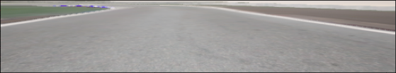
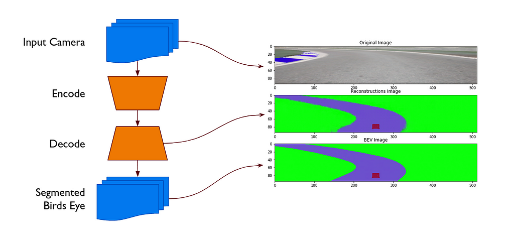
]]>Renukanandan Tumu*Autoencoder-based Perspective Transformation and Segmentation for Autonomous Racing2022-06-06T19:24:01+00:002022-06-06T19:24:01+00:00https://nandantumu.com/blog/2022/autoencoder-based-perspective-transformation-and-segmentation-for-autonomous-racingI want to share with you how I built a neural network to go from this: Input image from front camera of race car
To this:
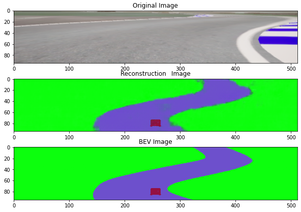
Output image, a segmented birds-eye view of the track. Race car in maroon, track in purple, off-track in green.
In words, our task is to take the input image, a front camera view of the track ahead, and construct a birds-eye view of the track instead, which has been segmented such that the track and off-track components are colored differently.
Extracting information about where the track is going to go is pretty difficult from just the input image, as a lot of our future track information is compressed into the top 20 pixel rows of our image. The birds-eye view camera is able to express that information about the track ahead in a much clearer format, one that we can more easily use to plan the behavior of the car.
This makes reconstruction task is important, because we will not always have access to the birds-eye view camera. If we can reconstruct these birds-eye images correctly, it allows us to plan with more clearly expressed information. An additional benefit is the dimensionality reduction we get. We are effectively representing the whole image as a set of 32 numbers, which takes up considerably less space than the full image. We can use this decreased dimensionality as an observation space for a Reinforcement Learning algorithm if we so desire.
We leverage past advances in a tool called Variational Autoencoders (VAEs), to help us accomplish this task. In plain English, we take the image, compress it down to a latent space of 32 dimensions, and then reconstruct our segmented birds-eye view. The exact network architecture is expressed in PyTorch code at the end of this article.
Overall pipeline of the Bird’s-Eye View Reconstructor
To train this, we collect a series of images from the car, both the front camera, as well as our bird’s eye camera. We encode them with the encoder, which is a series of convolution layers. Next, we drop the dimensionality to our target size with a fully connected layer. From this, we use the decoder to reconstruct our image with a series of deconvolution layers.
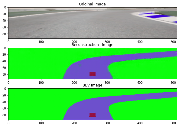
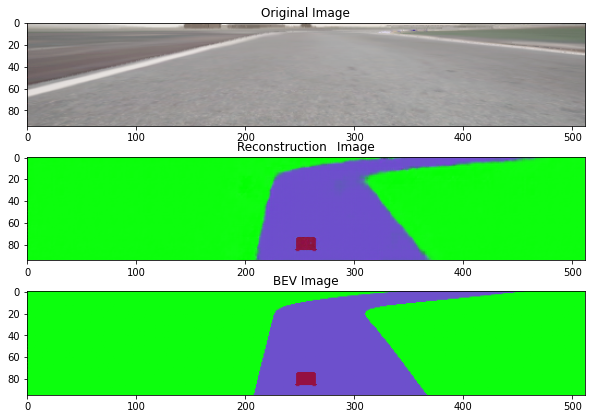
At the end, we have a method which is able to generate the reconstructions we see below!
Sample output, with input on top, ground truth on the bottom, and the reconstruction in the middle
While we can see some noise in the reconstruction, it captures the spirit and the overall curves of the track ahead quite well. Our team was able to use this method, as well as extensions to it to help us develop autonomous racing control methods in the AICrowd Autonomous Racing Challenge!
]]>Feature Scaling in Real Cardiac Electrograms2019-07-10T23:29:59+00:002019-07-10T23:29:59+00:00https://nandantumu.com/blog/2019/feature-scaling-in-real-cardiac-electrogramsFeature scaling is an essential part of any machine learning pipeline. In the process of designing our own neural networks designed to interpret EGMs, we have tested various scaling functions on real data, and we present the results below.
Functions Used:
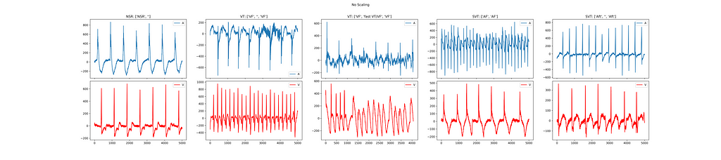
No Scaling — This retains the data in its raw format.
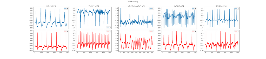
Min-Max Scaling — This function scales the maximum value to be 1, and the minimum value to be -1.
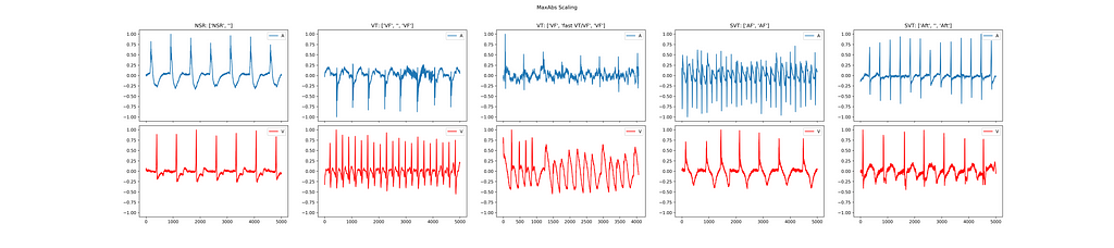
Max Abs Scaling — This function scales the maximum absolute value to be either 1 or -1.
Normalization —This function takes the L2 norm of the sample.
Power Transformation — Applies a monotonic transformation to the data. Monotonicity means that the function is always increasing, or always decreasing. In this case, the Yeo-Johnson method is used.
What do we want?
There are a few qualities we’re looking for in a good scaling algorithm.
Constant Range. We want to make sure the values after scaling, are put into the same range, in this case [-1,1].
Feature Extraction. We want features, or patterns, that exist in the data to become more evident.
Rough Equivalence. What I mean by this is that the data should end up in largely the same format after processing. When this Neural Network is deployed, it is important that data that is encountered in the wild follows the same general format as the data that the network trained on.
Impact of scaling methods on real electrograms
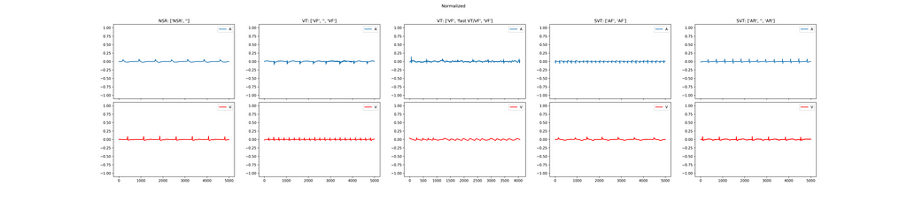
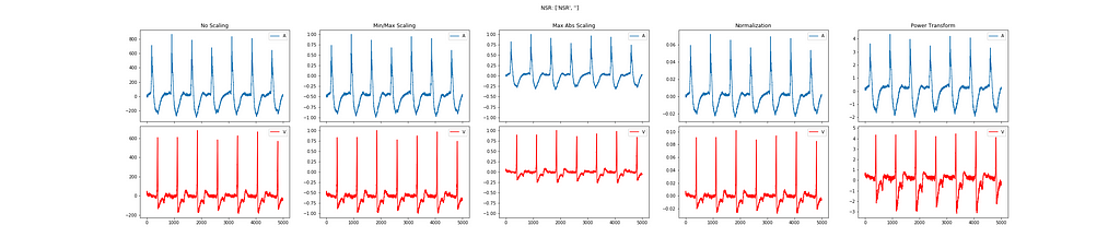
No Scaling
Unscaled EGMs
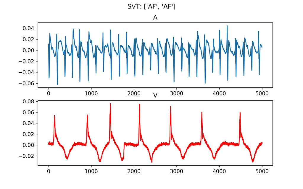
This is our baseline moving forward. The blue channel is a recording from the atrium of the heart, and the red is from the ventricle. The signals above are the original unscaled signals representing five conditions the heart is in. NSR means Normal Sinus Rhythm. VT stands for Ventricular Tachycardia, VF for Ventricular Fibrillation. VT and VF are potentially lethal. SVTs are a category of arrhythmia called Supraventricular Tachycardia. You can read more about them here. AF is Atrial Fibrillation and Aft is Atrial Flutter. SVTs are generally non-lethal.
Min Max Scaling
EGMs scaled so that the minumum value is scaled to negative one, and the maximum to one.
The Min Max scaled signals are not centered around zero. Not only are the signals not centered around zero, they aren’t even centered around a consistent value. The center is -0.5 for the atrial channel in the NSR electrogram. In the Atrial Fibrillation example’s atrial channel, the zero is around 0.25. This variability is not what we’re looking for in preprocessing data.
MaxAbs Scaling
EGMs scaled so that the maximum absolute value is one or negative one.
This transformation, while following the same basic format of Min Max scaling, fares considerably better. Because it only modifies the maximum absolute value to be one or negative one, it preserves the center around zero. The application of a single scalar also means the shape of the signal is preserved. It does well on our three goals, ensuring that the signal is within the same range, that features are preserved, and turns different episodes into signals with similar characteristics.
Normalization
EGMs that have been normalized.
Normalization isn’t usually applied to time-series data sets, but I thought it’d be interesting to see how it performed. As you can see, it does an interesting job. The figure on the left shows us some more detail. This transformation is similar to the MaxAbs transform, in that it preserves the center and shape of the data. Unfortunately, the magnitude of the signal is so small that changes are barely noticable. This scaling method doesn’t perform well at keeping features apparent due to its magnitude issues.
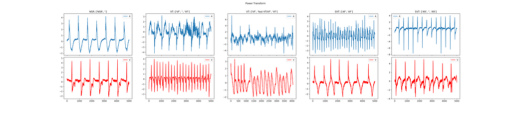
Power Transform
EGMs with a monotonic power transformation applied.
The power transform changes the shape of the signals. The best example of this is in the Normal Sinus Rhythm’s ventricular channel. The power transform magnifies the negative peaks of the signal. This could be very helpful in magnifying details that could be missed. Another benefit is that the signals appear to be centered around zero.
On the other hand, the signals are not bound by the same values. The max value ranges from 3 to 6. Perhaps applying MaxAbs scaling could turn this into a particularly powerful transformation.
Conclusions
It seems that Min Max Scaling and Normalization don’t perform well at all. The Power Transformation has interesting qualities, but doesn’t stand well on its own. The Max Abs scaling method, while very simple, provides all of the qualities we’re looking for.
All of the scaling methods applied to the NSR signal.
]]>Jun 25th 2019 Clinical Observations2019-06-27T12:14:38+00:002019-06-27T12:14:38+00:00https://nandantumu.com/blog/2019/jun-25th-2019-clinical-observationsToday, we had the privilege of observing the implant of one pacemaker and two ICDs at the Philadelphia VA Medical Center. The patients all had different underlying conditions, with each condition treated with a slightly different device and device setup. The patients were awake and anesthetized throughout the procedure.
Overall Process
Prep the patient
Cut a pocket in the upper left chest area, between the left pectoral muscle and the left deltoid.
Use a needle to find the axillary vein, with ultrasound sensing to visualize the needle in real time.
Put a wire through the needle tip, and into the vein to hold the place.
Repeat steps 3 and 4 for each catheter that is to be inserted.
Feed the catheter, which contains the leads, into locations in the heart
Test the sensing voltage, pacing voltage, and impedance of the leads.
Screw in or otherwise affix the leads. Right atrium and ventricular leads have a small screw which is used to fasten the lead to the myocardium. Left ventricular leads have small mechanical protrusions that keep the lead in place in the coronary sinus.
Retest the sensing voltage, pacing voltage, and impedance of the leads.
Plug the leads into the ICD or pacemaker
Place the device inside the pocket made in the skin
Close the pocket.
1st Procedure (~1hr)
The first procedure we observed was a dual-chamber pacemaker implant (DDDR). This was in response to paroxysmal complete AV block. This means that the patient had sudden onset cases where beats from the atrium would not conduct to the ventricles. The patient had episodes where ventricular beats were not observed for up to 8 seconds. The dual chamber pacemaker, is DDDR model. The first D means that it paces in both chambers, the second means that it senses in both chambers. The third D means that it does inhibition and triggered pacing, meaning it will not pace if it sees a natural beat, and pace if it notices a missing beat. The R means the algorithm is rate-responsive. The pacemaker will adapt the heart rate based on what it senses.
The two leads were standard bipolar leads, and were inserted through the vein in a fairly straightforward manner. The surgeons used tools called stylettes to change the way the leads moved through the heart. This device was made by St. Jude’s.
2nd Procedure (~3hrs)
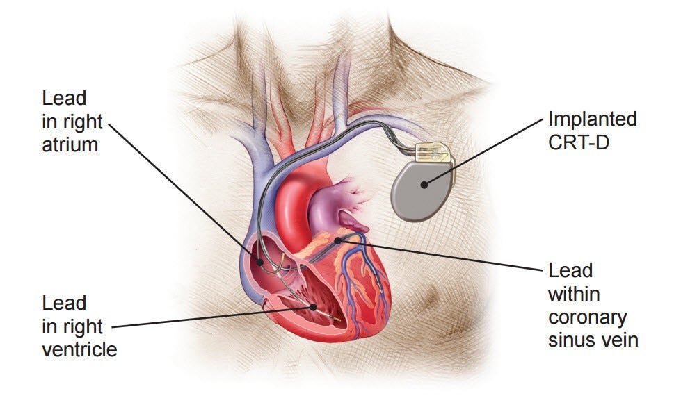
The second procedure was a CRT-D implant, manufactured by Biotronik. This was in response to LBBB or Left Bundle Branch Block. The patient also had a wider QRS complex on a surface electrogram. This happens when an atrial beat would be conducted through the right ventricle, but slow conduction of the signal to the left ventricle would result in an asynchronous beat. This patient was at risk for sudden cardiac death, which is why a CRT-D was implanted.
CRT-D devices have three leads, one in the right atrium, one in the right ventricle, and one in the left ventricle. The D refers to defibrillator, which means that the device can function as an ICD, which should prevent sudden cardiac death. The right atrium lead is identical to that used for the pacemaker. The right ventricle lead has a coil on it. That coil is used to deliver a defibrillating shock. The left ventricular lead is sent through the coronary sinus, near the tip of the left ventricle. This lead has four poles.
For sensing and pacing, a pole must be chosen, and a bipole configured. During the selection of a pole, pacing delivered from the L1 pole, or the farthest pole on the lead, closest to the “tip” of the heart, caused the patients diaphragm to contract. This was due to electrical activation of the phrenic nerve. L2 was chosen because a vector from the right ventricular coil to L2 would not generate a diaphragm response.
Credit: Boston Scientific
3rd Procedure (~1hr)
The implant was for a dual-chamber ICD, made by Medtronic. The patient exhibited signs of cardiomyopathy, with an ejection fraction of less than 35%. This means that on each heart beat, less than 35% of the volume of blood in the heart is expelled. The doctors postulated that it could be caused by AV block, and so opted to install a dual chamber ICD. This only required a right atrial and ventricular lead. This procedure was very similar to the implant of the dual chamber pacemaker that was done in the first procedure.
We’d like to thank the physicians, nurses, and OR team at the Philadelphia VA Hospital for graciously permitting our observation. We found it remarkably informational, and are grateful for the warm reception we received.
<hr><p>Jun 25th 2019 Clinical Observations was originally published in Medical CPS on Medium, where people are continuing the conversation by highlighting and responding to this story.</p>
]]>Supraventricular Tachyarrhythmias: An Overview2019-06-09T04:02:20+00:002019-06-09T04:02:20+00:00https://nandantumu.com/blog/2019/supraventricular-tachyarrhythmias-an-overviewThe purpose of this series on Supraventricular Tachyarrhythmias is to share what I’ve learned so far in my study, in the hopes that it may help someone else, perhaps in getting up to speed on the topic. Quick disclaimer: I’m still a beginner to the world of cardiology and electrophysiologic testing, so this may contain errors. Unless otherwise cited, the content of this series comes from a book entitled “Fogoros’ Electrophysiologic Testing”, by Dr. Richard N. Fogoros and John M. Mandrola.
Supraventricular Tachyarrhythmias are a group of arrhythmias that are non-lethal, and that occur above the ventricles, usually in the atria. They have the effect of increasing the heart rate. These tachycardia can be broadly divided into two classes, automatic and reentrant. We’ll talk about each one in turn, and the underlying mechanisms that make them possible.
Automatic Supraventricular Tachyarrhythmias
Automaticity triggering a second action potential. Diagram credit belongs to Fogoros et. al. Figure 1.3
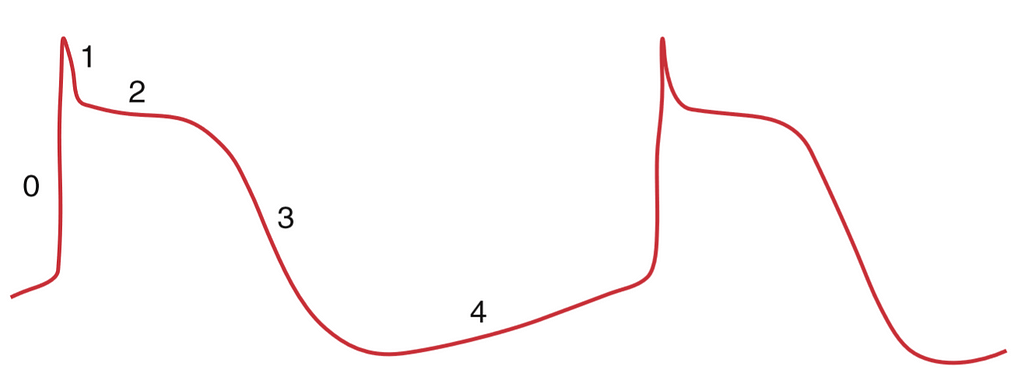
This class of tachyarrhythmias are made possible by misbehaving automaticity within the heart. Automaticity is a phenomenon where a cardiac cell, or more commonly, a group of them, has a leaky cell membrane, that triggers another action potential, “automatically”. This is represented in stage 4 of the figure. This phenomenon, when functioning normally, is what powers your heart’s pacemaker cells, and makes sure your heart continues to beat.
Automatic Atrial Tachycardia and Multifocal Atrial Tachycardia
Automatic Atrial Tachycardia (AAT) is caused by an additional pacemaker node, or automatic focus, in the atrial muscle wall, or myocardium. This additional automatic focus causes tachycardia, where its pacing is faster than that of the SA node.
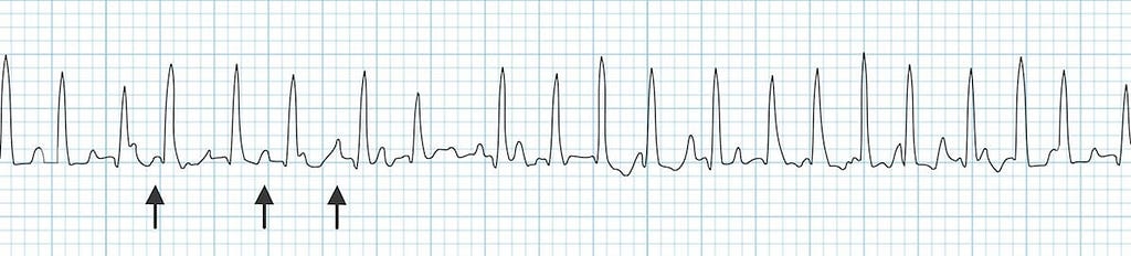
Multifocal Atrial Tachycardia (MAT) is much the same, except there are more automatic foci in the atrium. Each of the automatic foci fire independently, and this results in tachycardia. In MAT, the p-waves observed in a surface ECG look different, like in the image shown below.
Multifocal Atrial Tachycardia. The arrows point out discrete p-waves. Source: litfl.com
Inappropriate Sinus Tachycardia (IST)
This is a condition where the heart beats faster than normal, but for no apparent reason. The condition presents identically to Normal Sinus Tachycardia, with a major distinction being that there is no apparent reason for the tachycardia. Resting heart rates may be around 100bpm, and they increase even more on exertion. We are not sure what the cause of IST is, but it seems to frequently occur after a viral infection or physical trauma. It also appears to occur commonly in women in their 20s and 30s.
Reentrant Supraventricular Tachyarrhythmias
A reentrant circuit. Diagram credit belongs to Fogoros et. al. Figure 2.6
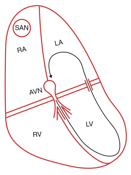
The mechanism of Reentrant Supraventricular Tachyarrhythmias is a reentrant circuit. Reentrant circuits, in the cardiac context, are circuits where a signal conducted across two different pathways may reenter the conduction pathway, resulting in a self-perpetuating cycle of signal conduction.
A core assumption here is that pathway A conducts slower, and has a shorter refractory period. Pathway B conducts faster, but has a longer refractory period. A signal that originates at the top of the diagram may conduct through both pathways. The signal conducted through A may reach conduct into B, which then continues conducting all the way through A again, creating a perpetual loop.
AV Nodal Reentrant Tachycardia (AVNRT)
In AVNRT, there are dual conducting pathways in the AV Node. The entire reentrant circuit exists in the AV Node.
A Bypass tract-mediated macroreentrant tachycardia circuit. Diagram credit belongs to Fogoros et. al. Figure 6.2
Bypass Tract-Mediated Macroreentrant Tachycardia
In Bypass Tract-Mediated Macroreentrant Tachycardia, the reentrant circuit goes through multiple regions of the heart, hence the macro prefix, and involves a bypass tract portion. This bypass portion could be created by a hereditary condition, like Wolff-Parkinson-White syndrome, or another bypass tract. These other bypass tracts are usually only functional in one direction, the retrograde direction.
Intraatrial Reentry
Intraatrial reentry occurs when the reentrant circuit is completely within the atria, and does not include the AV node at all. This type of reentrant circuit generates P waves that look different from the standard sinus P wave.
SA Nodal Reentry
Like the name implies, this reentry circuit is contained within the SA Node. This type of reentry is interesting in that it is spontaneously occurring, and Atrial Fibrillationdoes not exhibit the warm-up behavior that is usually observed with normal sinus tachycardia. The P waves it produces are identical to normal sinus P waves.
Atrial Flutter
Atrial flutter involves a reentrant circuit in the atria of the heart. It is kicked off by a premature atrial impulse, which “jumpstarts” the reentrant circuit. Atrial Flutter is often observed with 2:1 AV block, which means that 2 P waves are observed for every QRS complex. Atrial flutter can result in heart rates at or over 220 bpm.
Atrial Fibrillation
Atrial Fibrillation, or AFib, is a condition where atrial and ventricular activity is chaotic and uncoordinated. In the image below is an example of AFib where a P wave is not observable.
A diagram showing Atrial Fibrillation. Diagram credit belongs to Fogoros et. al. Figure 6.4
]]>Is Electricity Really Cheaper to Put in Your Car?2019-03-20T22:41:01+00:002019-03-20T22:41:01+00:00https://nandantumu.com/blog/2019/is-electricity-really-cheaper-to-put-in-your-carIs Electricity Really Cheaper than Gas?
How does the price of energy effect the economics of hybrid vehicles?
I was in the car with my dad, who drives a Chevy Volt, earlier this week. We were trying to decide if it would be more worth it to charge the car, or fill it with gas. The math we did in our heads pointed to gasoline being cheaper. Here’s a more formal analysis of what type of energy you should be putting in your car, by state.
Data Sources
I’m getting my gas price data from AAA, at this link. My electricity price data comes from the U.S. Energy Information Administration. Here’s a link. Data on the Chevy Volt’s mileage comes from fueleconomy.gov
Why the Chevy Volt?
You may be wondering if the Volt is a good car to be using for this analysis. Are other cars more efficient? I checked the EPA’s fuel economy numbers for all plug-in hybrids being sold in 2019, and only found two cars that do better than the Volt: the 2019 Toyota Prius Prime (25 kWh/ 100 mi), and the 2019 Hyundai Ioniq Plug-in Hybrid ( 28 kWh/ 100 mi). However, these cars do not have an electric only mode, they always run with gas. So using the Volt provides Plug-in hybrids the “benefit of the doubt” if you will.
Core Assumptions
Here are the core assumptions I’m making.
Mileage will be equivalent to the EPA’s fuel economy testing.
This means the car will get 100 miles on 31 kWh (Kilowatt hour), and 100 miles on 2.4 gallons
This equals 3.22 miles per kWh, and 41.66 miles per gallon.
Doing the Math
Let’s work through one state together. Let’s take my home state of Connecticut.
The electricity price is $0.2084 per kWh, and the price of gas is $2.63 per gallon.
Let’s calculate energy per dollar
The Kilowatt hours per dollar are $0.2084 ^-1 which equals 4.798.
The gallons per dollar are $2.63^-1 which equals 0.38
Let’s calculate the miles we get per dollar
For electricity, this is kWh per dollar * miles per kWh. This is 15.48.
For gas, this is gallons per dollar * miles per gallon. This is 15.87.
15.87 is bigger than 15.48, which shows us that you can travel further on a dollar if you buy gas in Connecticut than if you buy electricity.
What about the additional expense of hybrids?
Let’s go a step farther. The average miles driven by an average driver in the United States is 13,476. The source on that is the US Department of Transportation. Let’s figure out how expensive it would be to drive for a year with each of those energy sources.
We have a miles per dollar number, lets convert it to a dollars per mile number by taking its reciprocal.
For electricity, the dollars per mile number is 0.0646
For gas, the dollars per mile number is 0.0630
Let’s multiply it by the average number of miles driven to get an average fuel cost.
For electricity, the total fuel cost is $870.545
For gas, the total fuel cost is $848.988
Driving on gas saves you $21.55 per year!
What’s important here isn’t just that you would save $21.55 per year if you ran on gas over electric, but the price premium that electric vehicles command. Take for example the Hyundai Ioniq. The base level hybrid costs $21,400, and the plug-in hybrid costs $25,350. Both of these models are somewhat comparable to the Elantra, which costs $14,600. Let’s look at Honda. The Clarity Plug-in Hybrid costs $33,400, and a regular Civic costs $24,300. In both of these cases, we’re seeing a significant price premium for Plug-in vehicles. Electric vehicles must provide savings over gas vehicles to justify the higher price point.
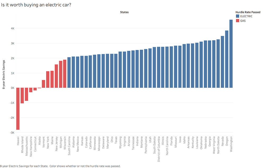
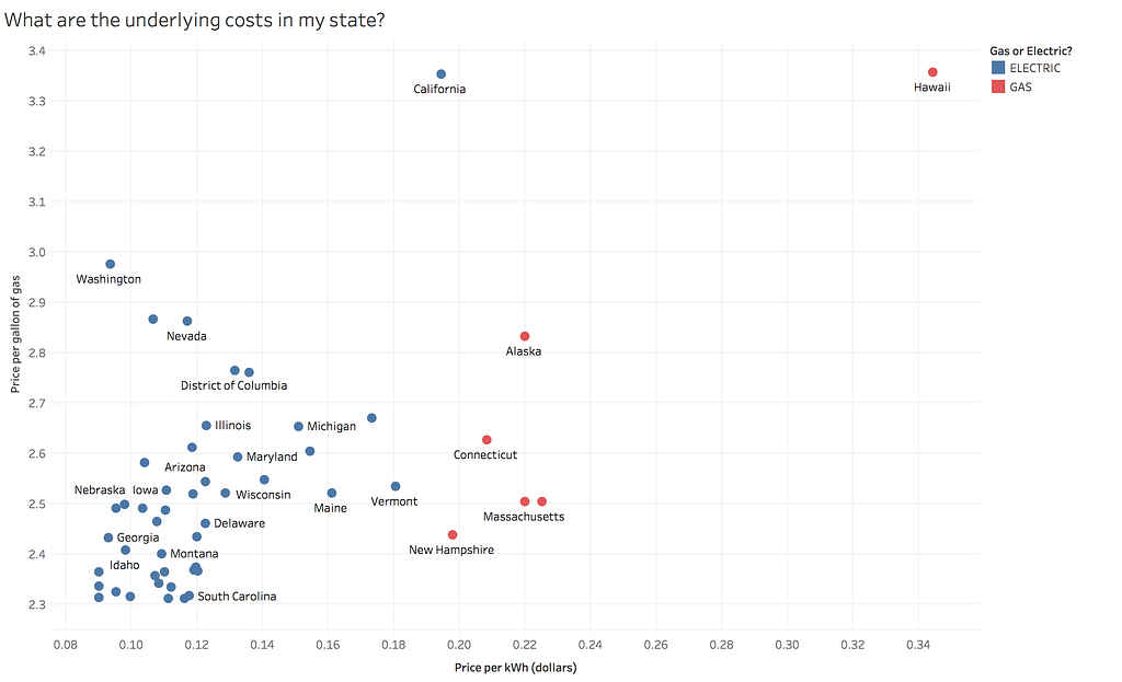
I’ve calculated the numbers for each state, and published the results below. In the second pane, you can set your own hurdle rate, to see if you’d break even in 8 years of car ownership. You can see how your state’s energy rates compare to others in the third tab of the visualization. Feel free to explore!
Check out the website above for Alaska and Hawaii, and more details.Check out the website to edit the hurdle rate for yourself.Can’t find your state? Check out the website.
Conclusion
There are six states where gas is cheaper than electric in this case. Alaska, Connecticut, Hawaii, Massachusetts,New Hampshire, and Rhode Island. There are a couple things of note here though. Gas prices are more variable than electricity prices, meaning at this time next year, gas may be significantly more expensive, while electricity prices remain the same. On the other hand though, electric vehicles and plug-in hybrids are more expensive than traditional gas powered cars. A hurdle rate of $5,000 is not cleared in any of the states in the USA. When companies like Tesla advertise gas savings as part of their prices, calculations like the ones we just performed take on a new importance. I think the 6 states above need to take a hard look at the cost of electricity in their states. Utility costs are a significant cost of doing business, and lowering them doesn’t just impact the economics of hybrids.